Usage¶

Here, it is assumed that one of the provided spectrograph HDF model files is used or that the appropriate model has been created from the ZEMAX file.

Basics¶

Echelle++ is controlled via command line arguments.

./echellesimulator -h

lists all available arguments.

This makes it easy for Echelle++ to be scripted. Look at the examples folder to see how Echelle++ can be called within python.

Example 1: Flat¶

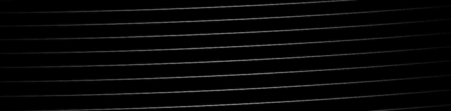
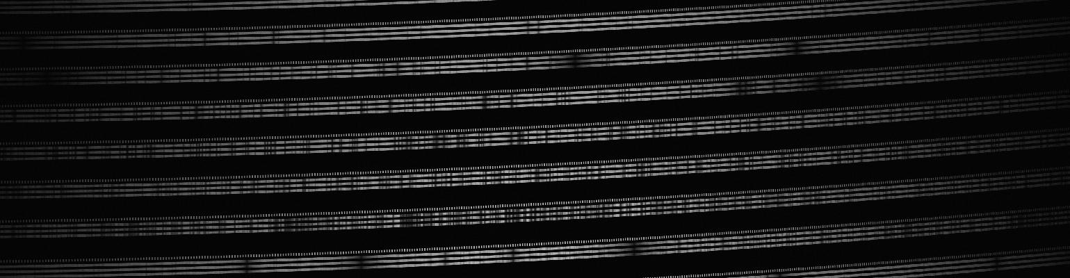
As a first example, we simulate a flat field. Or more precisely, we use a source of constant spectral density. The unit is µW/µm.

./echellesimulator --spectrograph MaroonX --constant 0.0001

Note

Since we didn’t specify the integration time manually, a default value of 1s is used.

The output will look like this (partly shown):

Note

Due to the photon-wise generation of the spectrum, all generated spectra naturally show photon noise.

For a high signal to noise (S/N) spectrum, increase the integration time or the spectral density.

Example 2: multiple fibers¶

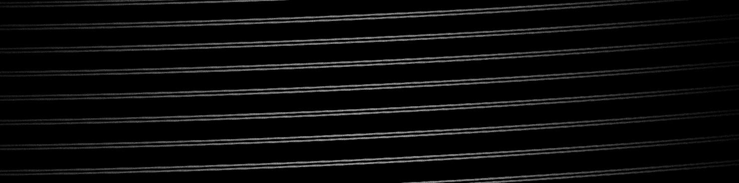
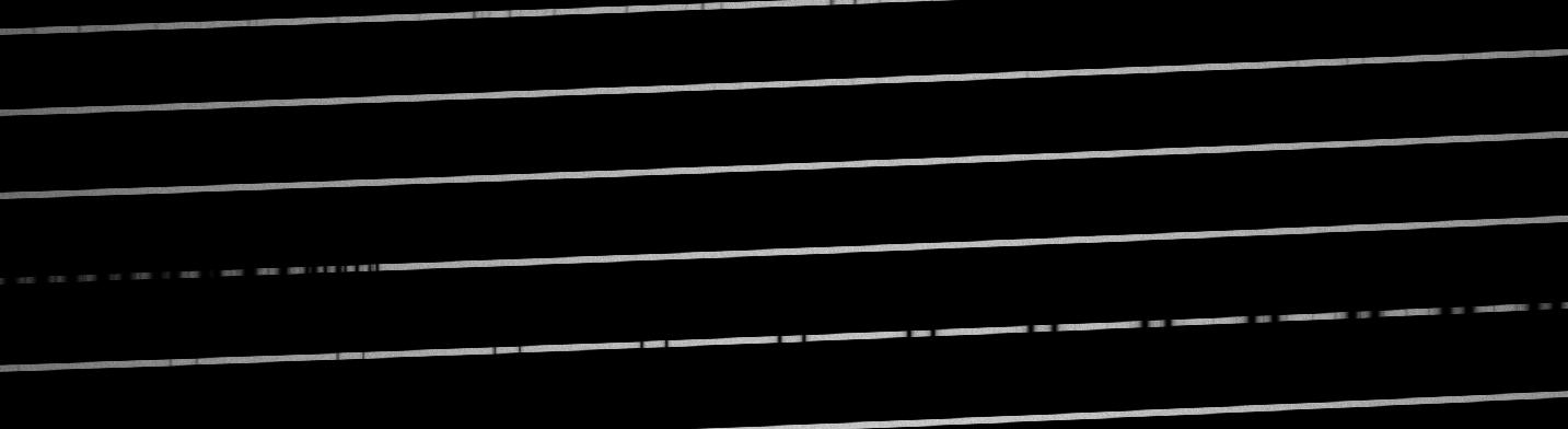
For multiple fiber spectrographs, we need one call to Echelle++ for each fiber. In the following example, we simulate a flat spectrum in the first two fibers of the MaroonX spectrograph.

./echellesimulator --spectrograph MaroonX --constant 0.001 -o flat2.fit
./echellesimulator --spectrograph MaroonX --constant 0.001 -f 2 -k 1 -o flat2.fit

Warning

The -k 1 flag of the second command makes sure that the content of flat2.fit will not be overwritten, but rather added to the current simulation. If the flag was not given, the second command would overwrite the file.

The output should look like this (partly shown):

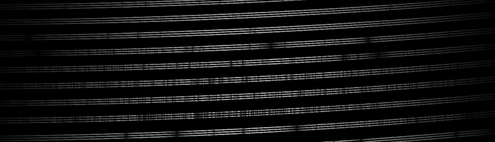
Example 3: A stellar source + RV shift¶

When simulating stellar sources, a visual magnitude of the source has to be provided. Also, a telescope size should be provided, otherwise, a default telescope of 1m diameter is used to calculate the photon flux. Here, we specify a telescope of 8.1m diameter and 128.12m focal length, a integration time of 60s. Our source is a simulated M-dwarf spectrum using the PHOENIX simulations with an effective temperature of 3500 K, Z=-1.0, alpha=0. and surface gravity of log_g=5.5. The V-band magnitude was specified to be 14. We also set the radial velocity to 50 m/s.

./echellesimulator --spectrograph MaroonX --telescope 8.1,128.12 --phoenix 3500,-1.,0.,5.5,14 -t 60 -r 50
./echellesimulator --spectrograph MaroonX --telescope 8.1,128.12 --phoenix 3500,-1.,0.,5.5,14 -t 60 -r 50 -k 1 -f 2
./echellesimulator --spectrograph MaroonX --telescope 8.1,128.12 --phoenix 3500,-1.,0.,5.5,14 -t 60 -r 50 -k 1 -f 3

Example 4: A line catalogue and readout noise¶

We can simulate line lists by providing a .csv file with the following column structure: “<wavelength>[micron];<intensity>[photons per second]” Consider the following excerpt of a Thorium line list

$more thar.csv

50004395; 6.9811
50005000; 9.2453
50006335; 18.3019
50007797; 12.0755
50012329; 2.8302
...

./echellesimulator --spectrograph MaroonX --linelist thar.csv -t 10 --bias 1000 --readnoise 5

Note

Here, it is assumed that thar.csv is located in the same folder as the executable.

Example 5: instrument efficiency¶

We can specify a wavelength dependent efficiency curve by providing a .csv file with the following column structure: “<wavelength>[micron];<efficiency>[fractional]”.

The following file will specify a 80% efficiency with a small section of 10% efficiency.

Intermediate values will be linearly interpolated.

$more efficiency.csv
4000;  0.8
5000;  0.8
6000;  0.8
6001;  0.1
6002;  0.1
6003;  0.8
9000;  0.8

./echellesimulator --spectrograph MaroonX --constant 0.001 --efficiency efficiency.csv

Example 6: simultaneous calibration¶

In the next example, we combine previous examples to generate a m-dwarf spectrum with an etalon as a simultaneous calibration source.

We add a radial velocity shift to both, the source and a different one to the calibration source.

We also add readout noise and a bias count.

Note

Only specify readout noise and bias once when simulating multiple fibers, since the signals get added otherwise.

./echellesimulator --spectrograph MaroonX --telescope 8.1,128.12 --phoenix 3500,-1.,0.,5.5,14 -f 2 -t 10 -r 50 -o example6.fit
./echellesimulator --spectrograph MaroonX --telescope 8.1,128.12 --phoenix 3500,-1.,0.,5.5,14 -f 3 -k 1 -t 10 -r 50 -o example6.fit
./echellesimulator --spectrograph MaroonX --telescope 8.1,128.12 --phoenix 3500,-1.,0.,5.5,14 -f 4 -k 1 -t 10 -r 50 -o example6.fit
./echellesimulator --spectrograph MaroonX --etalon 10,1.,0.,0.92,0.001 -f 5 -k 1 -t 10 -r -10.5 --readnoise 5 --bias 1000 -o example6.fit

Example 7: telluric contamination¶

In the last example, we include telluric contamination.

For now, we have to provide a .csv file containing the atmospheric transmission with the following column structure: <wavelength>[micrometer];<transmission>[fractional]

E.g.

$tail LBLRTM_2009_12_01_03_LasCampanas_AM1.5_transmission.csv
0999989798;0.9785330023
0999990798;0.9785817472
0999991798;0.9786300428
0999992798;0.9786779455
0999993798;0.9787258996
0999994798;0.9787731210
0999995798;0.9788205029
0999996798;0.9788674287
0999997798;0.9789135205

shows the last entries of a high-resolution atmospheric transmission spectrum.

Simulating a blackbody spectrum and providing the atmospheric model as an efficiency:

./echellesimulator -s MaroonXred --blackbody 4500,13 --telescope 8.1,128.15 --efficiency LBLRTM_2009_12_01_03_LasCampanas_AM1.5_transmission.csv

gives

Have fun !